While LLMs and their revolutionary transformer technology continue to impress us with new milestones, their foundations are deeply rooted in decades of research conducted in neural networks at countless institutions, and through the work of countless researchers.

Introduction

Large Language Models (LLMs) have gained momentum over the past five years as their use proliferated in a variety of applications, from chat-based language processing to code generation. Thanks to the transformer architecture, these LLMs possess superior abilities to capture the relationships within a sequence of text input, regardless of where in the input those relationships exist.

Transformers were first introduced in a 2017 landmark paper titled “Attention is all you need” [1]. The paper introduced a new approach to language processing that applied the concept of self-attention to process entire input sequences in parallel. Prior to transformers, neural architectures handled data sequentially, maintaining awareness of the input through hidden states that were recurrently updated with each step passing its output as input into the next.

LLMs are only an evolution of decades old artificial intelligence technology that can be traced back to the mid 20th century. While the breakthroughs of the past five years in LLMs have been propelled by the introduction of transformers, their foundations were established and developed over decades of research in Artificial Intelligence.

The History of LLMs

The foundations of Large Language Models (LLMs) can be traced back to experiments with neural networks conducted in the 1950s and 1960s. In the 1950s, researchers at IBM and Georgetown University investigated ways to enable computers to perform natural language processing (NLP). The goal of this experiment was to create a system that allowed translation from Russian to English. The first example of a chatbot was conceived in the 1960s with “Eliza”, designed by MIT’s Joseph Weizenbaum, and it established the foundations for research into natural language processing.

NLPs relied on simple models like the Perceptron, which were simple feed-forward networks without any recurrence features. Perceptrons were first introduced by Frank Rosenblatt in 1958. They were a single-layer neural network, based on an algorithm that classified input into two possible categories, and tweaked its predictions over millions of iterations to improve accuracy [3]. In the 1980s, the introduction of Recurrent Neural Networks (RNNs) improved on perceptrons by handling data sequentially while maintaining feedback loops in each step, further improving learning capabilities. RNNs were better able to understand and generate sequences through memory and recurrence, something perceptrons could not do [4]. Modern LLMs improved further on RNNs by enabling parallel rather than sequential computing.

In 1997, Long Short-Term Memory (LSTM) networks introduced deeper and more complex neural networks that could handle greater amounts of data. Fast forward to 2019, a team of researchers at Google introduced the Bidirectional Encoder Representations from Transformers (BERT) model. BERT’s innovation was its bidirectionality which allowed the output and input to take each other’s context into account. This allowed the pre-trained BERT to be fine-tuned with just one additional output layer to create state-of-the-art models for a range of tasks [5].

From 2019 onwards, the size and capabilities of LLMs grew exponentially. By the time OpenAI released ChatGPT in November 2022, the size of its GPT models was growing in staggering amounts, until it reached an estimated 1.8 trillion parameters in GPT-4. These parameters include learned model weights that control how input tokens are transformed layer by layer, as discussed later in this article. ChatGPT allows non-technical users to prompt the LLM and receive a response quickly. The more the user interacts with the model, the better the context it can build, thus allowing it to maintain a conversational type of interaction with the user.

The LLM race was on. All the key industry players began releasing their own versions of LLMs to compete with OpenAI. To respond to ChatGPT, Google released Bard, while Meta introduced LLaMA (Large Language Model Meta AI). Microsoft had partnered with OpenAI in 2019 and built a version of its Bing search engine powered by ChatGPT. DataBricks also released its own open-source LLM, named “Dolly”.

Understanding Recurrent Neural Networks (RNNs)

The inherent characteristic of Recurrent Neural Networks (RNNs) is their memory or hidden state. RNNs process input sequentially, token by token, with each step considering the current input token and the current hidden state to calculate a new hidden state. The hidden state acts as a running summary of the information seen so far in the sequence. RNNs understand a sequence by processing them word by word, while keeping a running summary of the words seen so far [6].

The recurrent structure of RNNs means that they perform the same computation at each step, with their internal state changing based on the input sequence. Therefore, if we have an input sequence x = (x1, x2, ..., xt), the RNN updates its hidden state ht at time step t using the current input xt and the previous hidden state ht-1. This can be formulated as:

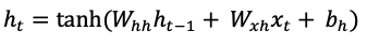
Where:

ht is the new hidden state at time step t
ht-1 is the hidden state from the previous time step
xt is the input vector at time step t
Whh and Wxh are the shared weight matrices across all time steps for hidden-to-hidden and input-to-hidden connections, respectively.
bh is a bias vector
tanh is a common activation function (hyperbolic tangent), introducing non-linearity.

This process can be visualized by breaking out the RNN timeline to show a snapshot of the system at each step in time, and how the hidden state is updated and passed from one step to the next.

Figure 1. An RNN through time. The RNN cell processes input and the hidden state from time t-1 to produce the hidden state that is used as input together with token input from time t.

Limitations of RNNs

The sequential nature of RNNs limits their ability to process tasks that contain long sequences. This may be one of the main limitations that gave rise to the development of the transformer architecture and the need to process sequences much faster and in parallel. The following are some of the main limitations of RNNs.

Limitations in modeling long-range dependencies: RNNs are limited in capturing dependencies between elements within long sequences. This limitation is due primarily to the vanishing gradient problem. As gradients (error signals) occur during later steps in time, it becomes increasingly more difficult for the signal to flow backwards to earlier time steps and adjust the weights. This is because the longer the sequence the fainter the signal becomes. As the signal becomes weaker, by the time it reaches the relevant steps it becomes increasingly more difficult for the network to learn and trace back the relationship between those earlier inputs and the later outputs.

Sequential processing: RNNs process sequences token by token, in order. Hidden states must also be processed sequentially such that to obtain the hidden state at time , the RNN must use the hidden state from as input. Modern hardware like GPUs and TPUs are well equipped to work with parallel computation. RNNs are unable to make use of this hardware due to their sequential processing, which leads to longer training times compared to parallel architectures.

Fixed size of hidden states: In the sequence-to-sequence model, the encoder must process and compress the entire input sequence into a single fixed size vector. This vector is then passed to the RNN decoder which is used to generate the output for the next hidden state. The compression of potentially long and complex input sequences into fixed-size vectors can be challenging. It also makes it difficult to retrain the network on all the input details that may have been compressed, and thus potentially causing some important information required for training to be missed.

How Transformers Replaced Recurrence

The limitations of RNNs in optimizing learning over large sequences and their sequential processing gave rise to the transformer architecture. Instead of sequential processing, transformers introduced self-attention, enabling the network to learn from any point in the sequence, regardless of distance.

Self-attention in transformers is analogous to the way humans process long sequences of text. When we attempt to translate text or process complex sequences, we do not read the entire text and then attempt to translate or understand it. Instead, we tend to go back and review parts of the text that we determine are most relevant to our understanding of it, so that we can generate the output we are trying to generate. In other words, we pay attention to the most relevant parts of the input that will help us generate the output.

Transformers apply global self-attention that allows each token to refer to any other token, regardless of distance. Additionally, by taking advantage of parallelization, transformers introduce features such as scalability, language understanding, deep reasoning and fluent text generation to LLMs that were never possible with RNNs.

How Transformers Pay Attention

Self-attention enables the model to refer to any token in the input sequence and capture any complex relationships and dependencies within the data [5]. Self-attention is computed through the following steps.

1. Query, Key, Value (Q,K,V) matrices

a. Query (Q): Represents what current information is required or must be focused on. This can be described by asking the question “What information is the most relevant right now?”

b. Key (K): Keys act as identifiers for each input element. They are compared against the input sequence to determine relevance. This is analogous to asking the question “does this input token match the information I am looking for?”

c. Value (V): Values are also associated with each input token and represent the content or the meaning of that token. Values are weighted and summed to produce the context vector, which can be described as “this is the information I have”.

The model performs a lookup for each Query across all Keys. The degree to which a Query matches a Key determines the weight assigned to corresponding Value. The model then calculates a weight or an attention score that determines how much attention a token should receive when generating predictions. The attention scores are used to calculate a weighted sum of all the Value vectors from the input sequence. The result is a vector containing the weighted sum of all the weighted value vectors.

Figure 2. Calculating the weighted sum vector. Attention scores are multiplied by the Value (input) vectors which are then summed to produce the weighted sum vector

We have already discussed how traditional RNNs may struggle to retain information for distant input due to the sequential nature of the hidden state. Attention, on the other hand, allows the model to consider the weights of all inputs and by summing them up. The resulting vector incorporates information from all inputs with the proper weights assigned to them. This allows the model to have a context of all input while focusing on the most relevant information in the sequence, regardless of their distance.

2. Multi-head attention

When we consider a sentence, we do not consider it one word at a time. Instead, we look at each specific word in the sentence whether it is the subject, the object or the overall grammar to make sense of the sentence and what it is trying to convey.

The same analogy applies when calculating attention. Instead of performing a single attention calculation for the vectors, multiple calculations are performed each on a single attention head, such that each head looks at a different pattern or relationship in the sequence. This is the concept of multi-head attention which allows the parallel processing of the vectors, allowing the model to look at different patterns or relationships within the sequence.

3. Masked multi-head self-attention

Masking ensures that the head focuses only on the tokens received so far when generating output, without looking ahead into the input sequence to generate the next token.

Attention score: The dot product of the and matrices is used to determine the alignment of each Query with each Key, producing a square matrix reflecting the relationship between all input tokens.
Masking: A mask is applied to the resulting attention matrix to positions the model is not allowed to access, thus preventing it from ‘peeking’ when predicting the next token.

Softmax: After masking, the attention score is converted into probability using the Softmax function. The Softmax function applies a probability distribution to a vector whose size matches the vocabulary of the model, called . For example, if the model has a vocabulary of 50,000 words, the output vector will have a dimension of 50,000. Each element in the vector corresponds to a score for one specific token in the vocabulary. The Softmax function takes the vector as input, and outputs a probability vector that represents the model’s predicted probability distribution over the entire vocabulary of the model for the current position in the output sequence.

Make it stand out

Whatever it is, the way you tell your story online can make all the difference.

4. Output and concatenation

The final step is to concatenate the output from all attention heads and apply a linear projection, using a learned weight matrix, to the concatenated output. The concatenated output is fed into another linear feedforward layer, where it is normalized back to a constant size to preserve the original meaning of the input before it continues to be passed deeper into additional layers in the network [6].

Conclusion

There is no doubt that transformers have revolutionized the way LLMs have been deployed and applied in a variety of applications, including chatbots, content creation, agents and code completion. By relying on large and ever-growing vocabularies, and an architecture that is designed for scalability and parallel computing, we are only beginning to discover the breadth of applications transformers can have.

As the challenges facing LLMs continue to be overcome, such as the ethical and environmental concerns, we can expect them to continue to become more efficient, more powerful and ultimately more intelligent.

While LLMs and their revolutionary transformer technology continue to impress us with new milestones, their foundations are deeply rooted in decades of research conducted in neural networks at countless institutions, and through the work of countless researchers.

References

[1] Ashish Vaswani, Noam Shazeer, Niki Parmar, Jakob Uszkoreit, Llion Jones, Aidan N. Gomez, Łukasz Kaiser, Illia Polosukhin. “Attention Is All You Need.” In Proceedings of the 31st Conference on Neural Information Processing Systems (NeurIPS 2017). arXiv:1706.03762 cs.CL, 2017

[2] The history, timeline, and future of LLMs

[3] Large language models: their history, capabilities and limitations

[4] RNN Recap for Sequence Modeling

[5] Transformer Explainer

[6] What is a transformer model?